SASpy manual

Written by A. Panjkovich.
Post all your questions about SASpy to the ATSAS Forum.

© ATSAS Team, 2016

Table of Contents

• Manual
  • Introduction
  • Installation
    • PyMOL installation
    • SASpy installation
  • Interface
• Examples
  • Interactive modeling
  • Automatic refinement

Manual

The following sections describe how to install SASpy plugin (and PyMOL) on different platforms and how to use the SASpy plugin.

If SASpy is useful for your research, please cite:
Panjkovich A. and Svergun D.I. (2016) SASpy: A PyMOL plugin for manipulation and refinement of hybrid models against small angle X-ray scattering data. Bioinformatics, 32, 2062-2064 DOI:10.1093/bioinformatics/btw071

Introduction

SASpy is a PyMOL plugin that provides a point-and-click interface for SAXS-based hybrid modeling using ATSAS programs. Different functions are available, such as theoretical scattering prediction, fits to experimental data, superimposition of low- and high-resolution models, manual and automatic refinement among others. SASpy was developed as a cross-platform alternative to MASSHA.

Installation

To use SASpy, both ATSAS and PyMOL need to be installed.

PyMOL installation

SASpy supports PyMOL 2.0, for which installers are available at https://pymol.org/2/ for Linux, Mac and Windows.

Alternatively, PyMOL is available free of charge as open-source at https://sourceforge.net/projects/pymol/. It can be downloaded and compiled.

Open source PyMOL can be installed on Linux and Mac simply through a package manager, for example in Ubuntu apt-get can be used as in sudo apt-get install pymol. In Mac, first install HomeBrew and then run brew install homebrew/science/pymol on a terminal.

Instructions for installing precompiled open-source PyMOL in Windows can be found at http://tubiana.me/how-to-install-and-compile-pymol-windows-linux-mac/.

Full details on PyMOL installation are available at the PyMOL wiki.

Note: Commercial and/or educational PyMOL binaries distributed by Schroedinger before the release of PyMOL 2.0 (Sept. 2017) may not work properly with SASpy. Please install a recent open-source version of PyMOL or PyMOL 2.0 for SASpy to work hassle-free.

SASpy installation

Once PyMOL and ATSAS are installed in the computer, SASpy needs to be added as a PyMOL plugin. For this, within PyMOL go to menu: Plugin, Plugin Manager, Install New Plugin and navigate to where the saspy.py file is located. In standard ATSAS installations, this will depend on the platform:

• Linux: /usr/share/atsas/pymolplugin
• Mac: /Applications/ATSAS/share/pymolplugin
• C:\Program Files\ATSAS-3.2.1 \bin\python3.7\site-packages\pymolplugins\saspy

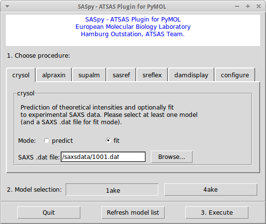
Alternatively, there is a copy of saspy.py at GitHub.

Restart PyMOL and the SASpy plugin should be available under the Plugin menu.

Note: ATSAS binaries need to be available in the PATH for SASpy to work correctly. If this is not the case, please edit your pymolrc file by adding the following line:

os.environ["PATH"] += os.pathsep + "/xxx/yyy/bin:"

where /xxx/yyy is the path to the local ATSAS installation.

Interface

The SASpy interface contains tabs, each corresponding to a different procedure. After choosing a procedure and its parameters, models can be selected and finally the Execute button needs to be pressed. Some tabs offer the possibility to select a SAXS .dat file, which will remain available for different procedures unless the user selects a different file.

Tabs have been named according to the ATSAS binary that provides their main functionality. The different procedures available are:

• crysol: theoretical scattering prediction and fit against SAXS data. Useful as well for manual hybrid modeling, as explained below.
• alpraxin: center model on the origin and align to coordinate axes.
• supalm: superimpose low- and high-resolution models.
• sasref: quaternary structure modeling and rigid-body refinement based on SAXS data.
• sreflex: flexible refinement of high-resolution models based on SAXS and normal modes.
• damdisplay: quick visualization settings for ab-initio DAM and beads models.
• configure: modify SASpy's settings.

Examples

Interactive modeling

In this example, we have collected SAXS experimental information for a protein complex. The atomic coordinates of individual subunits are known. We will combine the high-resolution models of the subunits with the SAXS data to generate possible models of the complex.

Loading models

PyMOL can automatically fetch models from the PDB server using the fetch command followed by the PDB id. For this exmaple, load both PDBs by typing the following commands in the PyMOL interface:

• fetch 1dksA
• fetch 1hcl
• zoom

Alternatively, structural models can be loaded using the PyMOL File - Open menu and navigating the filesystem.

Translating and rotating models

Right after loading the files, both subunits in this case are separated in space, the first step is to move them close together. One way to do this, is to change PyMOL's Mouse Mode from the default 3-Button Viewing to 3-Button Editing by clicking on the mode at the lower right corner of the PyMOL Viewer window.

Now, you can grab one of the subunits by clicking on it shift + middle mouse button and moving it closer to the other subunit. To rotate a single subunit, use shift + left mouse button. Once both subunits are arranged properly, the fit against experimental SAXS data can be checked using the crysol tab of SASpy as described below.

Evaluating the model fit against SAXS data

Open SASpy from the PyMOL plugin menu. Select crysol tab and click on the browse button availabe inside the tab to navigate to the complex.dat file provided in the examples directory. Once the SAXS data file has been loaded, use SASpy's model selection buttons to select both subunits. Once you click Execute, SASpy will write a PDB file containing the selected units in the orientations displayed on the screen. Then, the program CRYSOL will be run to check for the fit of the generated model against the selected SAXS data file. Once CRYSOL run completes, the resulting .fit file will be displayed and the obtained Chi-square value is reported on the PyMOL terminal. The generated files (.pdb, .fit, etc) are available in the working directory, which can be defined using the configure tab.

Alternative conformations can be tested by slightly moving one of the subunits in respect to the other as explained above, and then pressing the Execute button again.

Comparison against known complex structure

For this exercise, the structure of the protein complex is known crystallographically (PDB id 1buh), the user can fetch that structure to compare the manually built complex with the known complex. To superimpose the subunits to the known complex (and obtain the correct "answer"), type the following commands:

• fetch 1buh
• align 1dksA, 1buh
• align 1hcl, 1buh

Now, using these orientations for 1dksA and 1hcl, an excellent agreement should be obtained against the SAXS data when testing using the crysol tab.

Automatic refinement

The iterative process of manually rearranging the protein complex can provide good results, but automated refinement modes are available. A simple interface is provided to the SASREF program through the sasref tab. Two SASREF refinement modes have available through SASpy:

• local: quick search using limited translations and rotations of individual subunits. This mode is useful for small optimizations using the initial configuration as a starting point.
• global: in this mode, SASREF will run longer to explore a larger solution space, allowing large changes in position and orientation of subunits. In this mode, the initial configuration of the complex is not relevant.

Once SASREF finishes, the obtained complex is written to file and the new fit to the experimental SAXS data is provided. The subunits on the PyMOL display are rotated and translated according to the SASREF results.

For cases where conformational changes are expected to explain the discrepancy between a high-resolution model and SAXS data, the SREFLEX program can be used through SASpy's srelex tab. If a single model is selected, SREFLEX will attempt to subdivide the molecule into subdomains to improve the modeling of conformational change. If more than one model is selected, SREFLEX will consider these as independent domains for the initial refinement stages. Once the SREFLEX calculations finish, the obtained fits are displayed and the corresponding models are written to file and loaded in the current PyMOL session.