GNOM manual

Program written by D.I. Svergun, A. Semyenuk.

Documentation written by D.I. Svergun, A. Semyenuk and M.J. Gajda.
Post all your questions about GNOM to the ATSAS Forum.

© ATSAS Team, 1991-2009

Table of Contents

• Manual
  • Introduction
  • Running GNOM
    • Command-Line Arguments and Options
    • Interactive Configuration
      • Integral kernel and job type
      • Experimental conditions
      • Regularization parameter
      • Perceptual criteria
      • Error estimates
      • Graphics
        • Gnuplot graphics (UNIX version)
      • Next job
      • Interactive help
    • Runtime Output
    • Practical advices
  • GNOM Input Files
    • Scattering data
      • Standard deviations
    • Configuration file
    • Beam profile
  • GNOM Ouput File
• Examples
  • Lysozyme data

Manual

Introduction

GNOM is an indirect transform program for small-angle scattering data processing. It reads in one-dimensional scattering curves (possibly smeared with instrumental distortions) and evaluates the particle distance distribution function P(r) (for monodisperse systems) or the size distribution function D(R) (for polydisperse systems). The main equations relating the scattering intensity to the distribution functions and describing the smearing effects one can find in the text-books (e.g. [1]).

GNOM is similar to the known programs of Glatter [2], Moore [3] and Provencher [4]. There are, however, some points, which make GNOM more convenient in application. GNOM is a dialogue program; the user instructions presented here explain how to answer the questions properly. The versions E4.0 and higher make use of the "configuration file", where some or all the parameters can be pre-defined; this allows to work with GNOM in different modes, ranging from fully interactive to batch mode. The names of the parameters in the following description refer to the configuration file names.

The algorithms used in the program are described elsewhere [5-7]. They are based on the Tikhonov's regularization technique [8]; several subroutines published in [9] are modified and used in GNOM. The value of the regularization parameter is estimated by the program automatically using the perceptual criteria [10].

Running GNOM

Command-Line Arguments and Options

Use AUTOGNOM for automatic command-line driven functionality.

Interactive Configuration

Integral kernel and job type

The program searches for a distribution function in real space (characteristic function for monodisperse systems or size distribution function for polydisperse systems). These functions are related to the experimental intensity by corresponding Fourier transform followed by some convolutions representing smearing effects (if the latter exist). The integral equation is represented in a form of a linear system and solved with respect to the distribution function. The matrix of the system is called "design matrix". To evaluate it, the user must specify several parameters:

Prompt	Configuration variable	Applicability limits?	Value	Description
Angular scale				Scattering length units (s-units) used in input file:
			1	s = 4π*sin(θ)/λ, do not convert input data
			2	s = 4π*sin(θ)/λ, convert [nm-1] to [Å-1]
			3	s = 2*sin(θ)/λ [Å-1], convert to s = 4π*sin(θ)/λ [Å-1]
			4	s = 2*sin(θ)/λ [nm-1], convert to s = 4π*sin(θ)/λ [Å-1]
	JOBTYP		0	calculation of distance distribution function for a monodisperse system (default job). The function P(r) = γ(r)*r2 is evaluated, where γ(r) is the characteristic function of the particle.
			1	calculation of volume distribution function D(R)=(4*π/3)*R3 N(R) for polydisperse system of solid spheres (R is the sphere radius, N(R) relative number of particles with this radius in the system)
			2	calculation of size distribution function of particles with the user-supplied form factor (parameter FORFAC). In this case the form factor of particles should be supplied in a separate file. The form factor of particles should be supplied in a separate file.
			3	calculation of the distance distribution function of thickness assuming monodisperse system of flattened particles. The function P(r) = γt(r) is evaluated, where γt(r) is the characteristic function of thickness. In this case the experimental intensity as well the errors are multiplied by s2 which corresponds to the thickness scattering factor.
			4	calculation of the distance distribution function of the cross-section assuming monodisperse system of rod-like particles. The function P(r) = γc(r)*r is evaluated, where γc(r) is the characteristic function of thickness. In this case the experimental intensity as well as the errors are multiplied by s, which corresponds to the cross-section scattering factor.
			5	calculation of the length distribution function P(r) for a polydisperse system of long cylinders P(r) = H * N(H), where H is the length of the cylinder, N(H) number of rods of the lengths H. Radius of the cylinder is assumed to be a constant (see parameter RAD56 below).
			6	calculation of the surface distribution function P(r) for a polydisperse system of spherical shells P(r) = π*R2*N(R), where R is the outer radius of the shell, N(R) number of the shells of the outer radius R. The shells are assumed to have the same relative thickness (see parameter RAD56 below.)
	RMAX	JOB=0		Maximum diameter of the particle
	RMIN, RMAX	JOB=1		Minimum and maximum radii of spheres. Defines an interval in real space, where the distribution function is assumed to be non-zero.
	RMIN, RMAX	JOB=2		Minimum and maximum characteristic particle sizes. Defines an interval in real space, where the distribution function is assumed to be non-zero.
	RMAX	JOB=3		Maximum diameter of the particle thickness. Defines an interval in real space, where the distribution function is assumed to be non-zero.
	RMAX	JOB=4		Maximum diameter of the particle cross-section. defines an interval in real space, where the distribution function is assumed to be non-zero.
	RMIN, RMAX	JOB=5		Minimum and maximum heights of cylinders. Defines an interval in real space, where the distribution function is assumed to be non-zero.
	RMIN and RMAX	JOB=6		Minimum and maximum outer radii of shells. Defines an interval in real space, where the distribution function is assumed to be non-zero.
	RAD56	JOB=5 or 6		RAD56 means the relative thickness of a shell (its inner radius is RAD56*(outer radius). RAD56=0 means infinitely thin shells.
	NREAL			Number of points in real space, in which the distribution function will be specified (less than 72). Default number of NREAL is evaluated by GNOM in order to have reasonable ratio (number-of-data-points)/(number-of-parameters-to-be-found).
	LZRMIN, LZRMAX			They fix values of the distribution function to zero at the ends of the interval, if set to Yes.
	KERNEL			Kernel-storage file name, where the design matrix is saved.
Experimental conditions
	IDET			The user must define which type of experimental set-up is used:
			0	no smearing,
			1	1D-detector (slit geometry with rectangular slits is assumed),
			2	means 2D-detector (the data is obtained by a circular average).
	FWHM1, FWHM2	IDET=1 or 2		are the Full-Width-at-Half-Maximum of the wavelength distribution function for the first (second) data set. FWHM=0 means monochromatic radiation. If IDET=2 (2D-detector), a possibility of submitting an arbitrary wavelength profile is forseen. To this end, one should specify FWHM=0, and the program will try to read the wavelength profile from the beam profile file (SPOT1 and/or SPOT2), assuming that it follows the beam profile. If the wavelength profile is not present monochromatic radiation is assumed.
Beam divergence in 1D case				The beam profile is assumed to be a trapezoidal function.
	AH1, AH2	IDET=2		projection of the beam height in the detector plane - respectively for dataset 1 and 2,
	AL1, AL2	IDET=2		half of the height difference between top and bottom edge of beam projection on the detector,
	AW1, AW2	IDET=2		projection of the beam width in the detector plane - respectively for dataset 1 and 2,'
	LW1, LW2	IDET=2		half of the width difference between top and bottom edge of beam projection on the detector,
Beam divergence in 2D case
	SPOT1 and SPOT2	IDET=2		To describe the beam divergency in the 2D-case the used should specify the file containing the "spot function", i.e. distribution of the primary beam intensity in the 2D-detector plane (without sample), measured with the given geometry. The function is assumed to be a square matrix, stored in a separate file.

Regularization parameter

The main question, typical for solving ill-posed problems is how to stabilize the solution properly (here: how to find a positive regularization parameter ALPHA, which demands smoothness of the solution). The larger ALPHA, the more attention is paid to the smoothness of the distribution function and the less attention - to fitting the experimental data.

This search was done in the earlier GNOM versions by the generalized discrepancy method [8] using successive calculations with different ALPHA values. The ALPHA was chosen so as to fulfill the well-known χ-square criterion: the sum of deviations of the smeared intensity, corresponding to the given ALPHA, from the experimantal values, weighted with the standard deviations, should be equal to 1 + AN1. Here the value of AN1 is calculated by the program and represents the degree of unconformity of the problem (it equals to zero if NS=NR and increases with the ratio NS/NR). If AN1 is too large (AN1 > 1) the warning is printed. This warning, in principle, means that the input data/parameters are to be checked; however, it does not hinder following calculations.

The discrepancy criterion alone, however, in many cases can not ensure the correctness of the solution. Standard deviations may not be known or may be wrong. Another criterion which can also be used is the stability of the solution with respect to changing ALPHA. It can serve for manual [2], or automatic [6] search, but sometimes fails as well.

Perceptual criteria

In the EN.N versions the computer is instructed to get a plausible solution basing on several criteria, like its smoothness, stability, absence of systematic deviations, etc. Some of them are to be fulfilled by increasing ALPHA, the others - by its decreasing. A compromise is to be found. It is done as follows.

Each criterion is expressed mathematically. For a given solution one calculates the value of the criterion and compares with its ideal value. All estimates of the parameters have the form of Gaussians
P(i) = e^{-[(A(i) - B(i))/_σ(i)]2}
where:

A(i)

expected ("ideal") value of the criterion

B(i)

its actual value

σ(i)

width of the distribution (FWHM/1.665)

(values A(i) and σ(i) are specified a priori). Then the total quality estimate is calculated as

TOTAL = P = ΣP(i)*W(i) / ΣW(i)

where:

W(i)

weight of the given criterion (also fixed).

Therefore, all P(i) and P are between 0.0 and 1.0. The program searches for a maximum of the total quality estimate P.

The following criteria are used for estimates:

Estimate code	Description
DISCRP	χ-square test in reciprocal space - using the specified standard deviations. If they are correct, should be slightly less than 1 (ideal value is taken as 0.7). Increases with ALPHA.
OSCILL	shows the smoothness of the solution. Evaluated as the ratio ||dp / dr||  /  ||p|| related to this ratio for a monomodal sine function. Decreases with ALPHA. Ideal value 1.1 (for a characteristic function of a uniform sphere). Here || || denotes the function norm.
STABIL	shows stability of the solution with respect to the change of ALPHA. Calculated as d(ln||p||)/d(ln(ALPHA)). Ideal value 0.
SYSDEV	indicates the presence of systematic deviations of the restored (smeared) curve Ires(s) from the experimental data Iexp(s). Calculated as N1/(N/2), where N is the number of experimental points, N1 - number of changing sign of the difference (Iexp - Ires). Ideal value 1. Important parameter (unless you suspect your data contain systematic deviations). Increases with ALPHA.
POSITV	relative norm of positive part of P(r). Ideal value, of course, 1.
VALCEN	indicates validity of the chosen interval in real space (relative norm of the central part of P(r) ). Ideal value tends to 1 (0.95 for a sphere). Much less than 1 if your interval is too wide.

The user is asked to enter the ALPHA value. If this value is already known to the user (e.g., from previous calculations with similar data), he can type the negative ALPHA, then the solution with -ALPHA will be evaluated. A positive ALPHA means automatic search of ALPHA by maximizing the total quality estimate as described below; no further manual refinement is possible (this is convenient for using GNOM in the batch mode). Default case (ALPHA=0) means automatic search accompanied by a graphic representation (plot lg(ALPHA) vs TOTAL estimate). This plot would help the user to correct ALPHA manually in the cases when the automatic search breaks down (see Practical advices).

The search of ALPHA works as follows. First the program finds the theoretical maximum (highest) ALPHA value for the given problem [7] (in graphic representation the Y-axis is drawn through this value). Then it tries to maximize the total estimate with the given set of A(i), σ(i) and W(i). The default set is:

Note that parameters OSCILL, STABIL and SYSDEV are considered to be most important.

The program evaluates first the grid of the TOTAL values for ALPHA < 1000*highest ALPHA (indicated as open circles in the plot). Then the golden section search is performed to maximize the estimate (characters '+' on the plot).

Note: when OSCILL is too large while SYSDEV already reasonable (here: OSCILL>13, SYSDEV>0.5), the value of TOTAL is put to zero. If zero value is encountered, the program stops evaluating the grid. This is made in order to avoid useless computations for too small ALPHA values.

After the solution is found, the user may either accept it, or change the weight/width of distribution for any criterion, or try to get a new maximum estimate, or change the ALPHA manually. When you increase the distribution width for a given parameter, larger deviations from the expected values are allowed for this parameter. When you increase the weight of a parameter, it plays a more significaht role in the estimate, therefore the solution maximizing the estimate will be shifted to fulfill the corresponding criterion. The changed set of parameters can be stored onto an ASCII disk file and then used The solution can also be plotted on the screen. The intensity plot presents together the experimental data (astericks), the desmeared (solid) curve and the corresponding smeared (dotted) curve. Note that for the cases JOB=3, 4 and 5 the experimental curves are modified. Namely, for JOB=3, I(s) is multiplied by s², for JOB=4 by s, for JOB=5 divided by (2*J1(s*RAD56)/s*RAD56)² (the latter is the cross-section factor of a cylinder, J1(x) Bessel function of the 1-st order). These modified curves are are plotted and printed onto the output file.

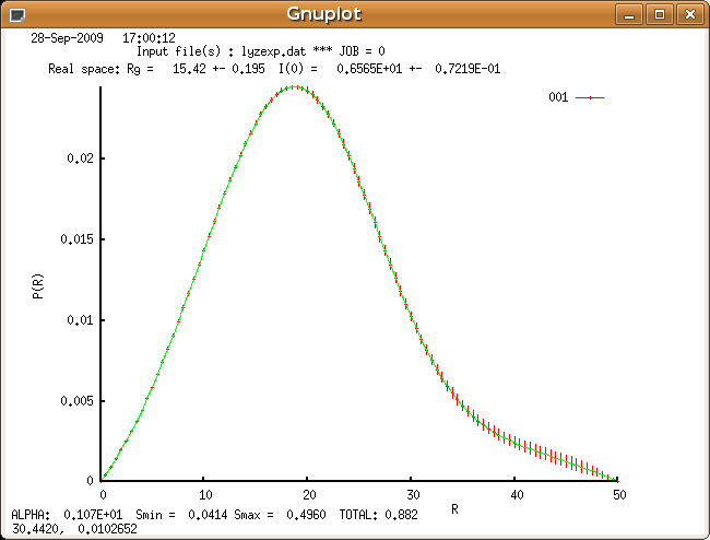
The distribution plot shows the obtained correlation or size distribution function. Radius of gyration and zero angle intensity are also evaluated in real space using the P(r) function. Note that for the case JOB=2 the values in real and reciprocal space may not coincide, because I(0) will be evaluated as the NDIM-th moment of D(R), and R_g as sqrt((NDIM+2)th moment)/(2*I(0)))again for a similar object by entering its name when prompted 'File containing expert parameters' (parameter EXPERT). In this file user may also edit all the values (including ideal estimations).

Error estimates

After the soluton is accepted by the user, the errors propagation can be estimated. This is made via a series of Monte-Carlo simulations. The standard deviations in the p(r) function as well as in the radius of gyration and zero-angle intensity are evaluated. The random sequence is initiated by the four-digit value of current time (min:sec), so that slightly different values of error estimates are obtained on exactly the same data set (the number of Monte-Carlo generations is 100).

Note: the Monte-Carlo routines were rewritten for the versions E3.3 and then 4.1 therefore some differences may also exist between the results of different versions.

Graphics

Graphic routines in the program use MS-Fortran 5.1 graphic package (DOS/Windows version) or public domain Gnuplot package (UNIX version.)

Gnuplot graphics (UNIX version)

On UNIX machines, a possibility exists to use the public domain Gnuplot graphic package. It is used not as a separate interactive program, but as a graphic library. GNOM creates a sequence of data/command files in the /tmp directory which are then executed by Gnuplot. To use Gnuplot version of GNOM, Gnuplot version 3.0 and higher must be installed and the gnuplot executables should be in the PATH variable.

Next job

After the job is finished, the user is asked whether to run the program again (parameter NEXTJOB). Answering No stops the program. Yes means new job. Same means that the new data set will be calculated under the same conditions as the previous one (with the same integral kernel).

Interactive help

Answering a question mark ? followed by 'Enter' to each question allows to get a short help on the parameter.

Runtime Output

Runtime output format is identical to format of output file. It contains first alpha search history, then regularized curve, and finally P(r) distribution.

Regularized curve is printed in five columns:

Chord distribution function is printed in three columns:

Practical advices

This chapter has arisen as a result of practical applications of GNOM and is based mainly on the typical user questions.

GNOM is intended to be as user-friendly as possible, that is, it normally runs OK using the default answers. In particular, default value of the number of real space points is highly recommended to use.

The units in real and reciprocal space must be reciprocal to each other. Thus, if the momentum transfer is given in reciprocal Ångströms (Å^-1 for λ in Ångströms), the particle sizes in real space are to be specified also in Ångströms. If you want particle sizes in miles, the input file has to contain momentum transfer in reciprocal miles. The units of the parameters describing beam divergency should be the same as for the momentum transfer.

All the weighting functions are normalized so that the desmeared curve is on the same scale as the smeared one. In parcitular, as the wavelength effects are always relative, the wavelength distribution gets reduced to λ=1. This does not mean that the program works only for this wavelength, because the wavelength information is already contained in the s-units.

One more thing about the wavelength effects: in X-ray experiments with the conventional sources (X-ray tubes) they are normally negligible.

The rectangular slit geometry assumed for the 1D-detectors is normally a good approximation for practical applications. It is valid, of course, both for linear multi-channel detectors and single channel moving detectors. Note that the slit-height function, if non-symmetric, can be symmetrized, because of the properties of the slit-smearing integral. Asymmetries in the slit-width function, if exist, can be neglected, as the slit-width effects are normally small. The case of "infinitely long slit" can be covered, e.g., by putting AH=S_max, LH=0, where S_max is the momentum transfer of the last data point. For a more detailed description of the smearing effects see, e.g. Ref[1], Ch.9.

If you specify the maximum size so that D_max*S_min (S_min the momentum transfer of the first data point) is greater than π=3.1416926, a warning is printed. This means that the first data point is beyond the first sampling point and the information content may be not sufficient to obtain a reliable solution. However, the warning does not prevent the program from continuing.

Default settings of the EXPERT parameters are also valid for the most of normal systems. However, in some cases it is advisable to change the default set in order to ensure reliable automatic search of ALPHA. Typical examples are:

• If you do not know standard deviations in the experimental data, put the weight of DISCRP to zero.
• If you suspect that your distribution function is non-monomodal, put the ideal value of OSCILL to M, where M is the number of modes. For example, if you expect to have a bimodal size distribution function (JOB=1), put OSCILL=2.
• If the distribution function can show negative peaks (say, X-ray scattering from lipoproteins in water, JOB=0), put the weight of POSITV to zero (and OSCILL is better to put to 2 or 3, as in previous example).

The program may fail to evaluate the constant for the second run in the trivial case with no smearing because of poor stability of the design matrix in this case. The users are kindly asked to correct the value manually.

The program explores the range
(10³ * highest ALPHA) > ALPHA > (10^-18 * highest ALPHA)

to maximize the estimate. If the total estimate is monotonous in this range, the warning is printed. In such cases the user can perform manual search, or restart the maximization from the current point. Important note: normally, the plausible range of ALPHA is approximately 10-6 * (highest ALPHA).

If the solution found by the program is by far not acceptable, this just means that the maximization procedure (golden section search in logarithmic ALPHA scale) is trapped by a local minimum. One can restart the maximization from an ALPHA in a plausible range.

Another reason of getting a non-acceptable solution could be a non-consistency of the data and the assumptions. In this case the user will get the warning about AN1 and, normally, rather low value of the maximum estimate.

By default, the program puts P(RMIN)=0, P(RMAX)=0. If these conditions are not applied, non-zero P(r)'s can exist at the ends of the real space interval. Sometimes by P(0) one can take a constant background into account (note that for JOB=3 P(0) is normally non-zero). If you do not know D_max, it is better first not to fix P(RMAX), because this value will help to judge whether the chosen interval is correct (if, for example, RMAX is too small, P(r) is systematically higher than zero in the vicinity of RMAX).

Model calculations show that the evaluation of the size distribution function of cylinders (JOB=5) is a very ill-posed problem, because the scattering curves from long cylinders are rather flat and it is not so easy to distinguish between them in the scattering curve, as e.g. for polydisperse system of spheres. Therefore for JOB=5 it is very important to have good measurements in the beginning of the scattering curve where scattering from cylinders of different length differs significantly from each other.

GNOM Input Files

Scattering data

Input file (parameter INPUT1) is a sequential ASCII file containing the experimental data. The first line is always treated as a problem title (comment). Then the program searches for the first data line. Valid data lines should contain momentum transfer, non-zero intensity, and, optionally, standard deviation in a free format (that is, separated by blanks or commas). After this all valid lines are treated as data; invalid line or end-of-file are considered as the end of the input stream. The maximum number of data points is 1024.

This way to read data is rather flexible, allowing to skip additional headers and to use the data with or without the standard deviations.

With modern devices one can measure lots of data points with tiny angular step. This is not always good, and sometimes might become harmful when using indirect methods, because each angular point gives rise to a separate equation, which are, in fact, linearly dependent. Note that the angular step δ(s)=^D_samp/₆, where ^D_samp=(π)/_Dmax is a sampling distance, is claimed to be optimum. To optimize the performance, GNOM joins neighbouring data points when it finds the number of points to be unreasonably high.

The program can handle simultaneously two data sets corresponding to the same sample but recorded with different conditions (see below). The second input file (parameter INPUT2) should have the same structure. Default answer to the question 'Input file name, second run' is no second run.

Note, that the momentum transfer is assumed to be
s = 4 (π) sin (Θ) / (λ_average),
where Θ is a half of the scattering angle.

Example of the input file :

   PROBLEM #13
This line is skipped because of error, the next because of zero intensity :
  0.0001     0.0         17.1
This is again skipped: the next is the first valid data line:
 0.05564   ,     1.2323e10  111111111.
 0.05574 1.1323e10
 0.05584 18303353, 1e10 , This is the text which does not change anything!
  1.e-1     1.0323e10,   8E8    It is just not read.
  0.07        0.0         17.1
The previous line indicates the end of the data set

Standard deviations

If some standard deviations (or all of them) are not specified, negative or equal to zero, the user will be prompted for their estimation (parameter DEVIAT). A positive number means constant relative deviation per point. If the user enters zero (default answer), the program will estimate the errors automatically with the help of a polynomial smoothing procedure.

Giving 3 means that for each point with a non-positive standard deviation a relative deviation 0.03*I(s) is assumed, where I(s) is the intensity in this point.

Configuration file

Some or all of the parameters used by the program can be specified in the configuration file named 'gnom.cfg'. The first line of the file is always treated as a comment. The structure of a valid information line is shown below:

  1-7   9    Between brackets               Comment
 NAME  Type     Value
PRINTER C [      HPPCL       ]  Printer type

Here NAME is the name of the parameter (all names are fixed), the letter in the 9-th column shows the type of the parameter: (C - character, I - integer, R - real). The value of the parameter is to be put between the square brackets (not more than 35 characters). If the line is not valid (e.g., ] is missing, or the parameter name is wrong), it is skipped and the warning is printed. When GNOM is started, it first tries to find and read the configuration file in the current directory. If the local file named 'gnom.cfg' does not exist, it tries to read the global configuration file:

• On Windows PC, it is always the file 'c:\gnom\gnom.cfg'
• On UNIX machines, it is ${GNOCFG}gnom.cfg, where ${GNOCFG} is an environment variable. Example: if the command

     %setenv GNOCFG /usr/local/include/
  

  is given, the global configuration file is '/usr/local/include/gnom.cfg'

If GNOM finds a non-blank value between the square brackets for a parameter in the configuration file, this parameter is assumed to be already defined, therefore, it will not be prompted interactively (the other parameters will be asked as usual). The read-in configuration table is printed on the screen ( ... means that the variable is not defined). The user can either accept the values or switch to the interactive mode. GNOM assumes the interactive mode also when neither local nor global configuration file has been found.

Specific values for some parameters :

• Zero values of the parameters NREAL and COEF mean that the values evaluated by the program will be accepted.
• For the EXPERT and INPUT2, 'none' means no file.
• As UNIX is case-sensitive, be careful with the file names in the configuration file for the UNIX version.
• For IDET=2, if FWHM1/FWHM2 are equal to zero, GNOM will try to find the wavelength distribution function after the beam profile in the corresponding SPOT1/SPOT2 file.

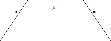
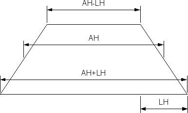
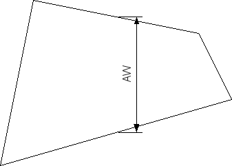
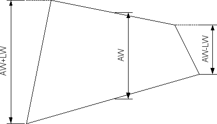
The example of the global configuration file is shown below. In this file only a few variables are fixed, and the program will not ask for them. More specific configuration files can be put in the local working directories. They can be configured in such a way, that the program will ask only a few questions or even run in the batch mode. Examples of the local configuration files can be found in the distribution package.

General configuration file

PRINTER C [      HPPCL       ]  Printer type
FORFAC  C [                  ]  Form factor file (valid for JOB=2)
EXPERT  C [     none         ]  File containing expert parameters
INPUT1  C [                  ]  Input file name (first file)
INPUT2  C [                  ]  Input file name (second file)
OUTPUT  C [                  ]  Output file
PLOINP  C [       y          ]  Plotting flag: input data (Y/N)
PLORES  C [       y          ]  Plotting flag: results    (Y/N)
EVAERR  C [                  ]  Error flags: calculate errors   (Y/N)
PLOERR  C [       y          ]  Plotting flag: p(r) with errors (Y/N)
LKERN   C [                  ]  Kernel file status (Y/N)
JOBTYP  I [                  ]  Type of system (0/1/2/3/4/5/6)
RMIN    R [                  ]  Rmin for evaluating p(r)
RMAX    R [                  ]  Rmax for evaluating p(r)
LZRMIN  C [                  ]  Zero condition at r=RMIN (Y/N)
LZRMAX  C [                  ]  Zero condition at r=RMAX (Y/N)
KERNEL  C [                  ]  Kernel-storage file
DEVIAT  R [      0.0         ]  Default input errors level
IDET    I [                  ]  Experimental set up (0/1/2)
FWHM1   R [                  ]  FWHM for 1st run
FWHM2   R [                  ]  FWHM for 2nd run
AH1     R [                  ]  Slit-height parameter AH (first  run)
LH1     R [                  ]  Slit-height parameter LH (first  run)
AW1     R [                  ]  Slit-width  parameter AW (first  run)
LW1     R [                  ]  Slit-width  parameter LW (first  run)
AH2     R [                  ]  Slit-height parameter AH (second run)
LH2     R [                  ]  Slit-height parameter LH (second run)
AW2     R [                  ]  Slit-width  parameter AW (second run)
LW2     R [                  ]  Slit-width  parameter LW (second run)
SPOT1   C [                  ]  Beam profile file (first run)
SPOT2   C [                  ]  Beam profile file (second run)
ALPHA   R [      0.0         ]  Initial ALPHA
NREAL   R [       0          ]  Number of points in real space
COEF    R [                  ]
RAD56   R [                  ]  Radius/thickness (valid for JOB=5,6)
NEXTJOB C [                  ]

The configuration file may contain arbitrary number of parameters. Not all of them have to appear in the file: the missing parameters will be treated as non-defined. It is advisable, however, to end the configuration file with the NEXTJOB parameter. If NEXTJOB is 'Y' or 'S', the next lines will describe the parameters for the new job, and so on. The last line in this case should be:

NEXTJOB C [ N ]   Ends the program

If you run the NEXTJOB, GNOM keeps the values which were used in the previous job as program defaults (for character variables only first 12 characters are kept).

Example: using the general configuration file shown above, the default output file will be 'gnom.out' (program default); if you enter another name, say,'mygnom.out' and then answer "Y" to the NEXTJOB question, default output file will be 'mygnom.out'.

Form factor of particles

The form factor of particles should be supplied in a separate file. The first line of this file should contain three values in free format:

This should be followed by the form factor values - NFORM of values in 8E10.3 format, NFORM<2500.

The function D(R) = N(R)*R^NDIM is evaluated; R is a user-defined characteristic size (e.g. radius of gyration.)

Beam profile files

Beam profile files are named in parameters SPOT1 and SPOT2, valid for IDET=2.

To describe the beam divergency in the 2D-case the used should specify the file containing the "spot function", i.e. distribution of the primary beam intensity in the 2D-detector plane (without sample), measured with the given geometry. The function is assumed to be a square matrix, stored in a separate file.

NB and TRANS can be written in the free format separated by blanks or commas (NB is compulsory parameter, TRANS - auxiliary). A comment can be added after TRANS (of NBEAM if TRANS is not specified).

All lines from 2nd on to (NB+1)st each contain NB numbers, separated by blanks or commas - beam profile.

The beam profile is used to evaluate the smearing due to beam divergency assuming that the curve is obtained by a circular average. Circularly averaged and normalized profile is used to this end. Additional smearing due to the radial average of the 2D-data is assumed to be one unit in the detector profile.

If FWHM = 0 and the wavelength profile is not submitted (or improperly specified), no wavelength smearing is included.

  7   1.5   Beam profile: Detector step=1.5*Delta(s) in the input file
      0.     1.     4.     5.     4.     1.     0.
      1.    45.   143.   211.   143.    45.     1.
      4.   143.   460.   678.   460.   143.     4.
      5.   211.   678.  1000.   678.   211.     5.
      4.   143.   460.   678.   460.   143.     4.
      1.    45.   143.   211.   143.    45.     1.
      0.     1.     4.     5.     4.     1.     0.
Wavelength profile (will be read in if FWHM=0 has been specified)
27, 4.59, 0.01106
0.00,  30.36, 68.16, 175.4, 236.1, 240.3, 200.3, 174.7,
139.2, 113.9, 112.4, 115.9, 109.3, 87.42, 65.51, 76.43,
116.7, 125.7, 128.0, 106.9, 80.50, 62.44, 48.11, 49.16,
43.41, 28.76, 0.

If instrumental distortions (especially all of them) are present, the evaluation of the design matrix may become a time-consuming procedure. When making successive computations with the same experimental conditions and real space limitations, one can use the same integral kernel, if it has been already calculated. For this, one should answer 'Y' when prompted 'Is the kernel already evaluated [N]?' (parameter LKERN), and enter after it the kernel-storage file name. The program can handle simultaneously two runs recorded at different (or the same) experimental conditions. The user should then supply two separate experimental data files (first - with lower s range; however, the ranges may overlap) and specify explicitly two sets of experimental conditions. The scale factor for the second run (parameter COEF) is evaluated by the program automatically [7].

GNOM Output Files

This is a sequential disk file where all the information from GNOM will be printed in ASCII form (parameter OUTPUT, default file name is gnom.out.)

Examples

Lysozyme data

Input data for lysozyme is in file lyzexp.dat. It has D_max of 50. You may give default answers to other questions. (Non-default answers are marked below in italic.)

                - - - - - - - - - - - - - - - - - - - - - - - - -
           G N O M  ---  Version 4.5a revised 09/02/02
   Please reference: D.Svergun (1992) J.Appl.Cryst. 25, 495-503
                - - - - - - - - - - - - - - - - - - - - - - - - -
  Configuration file not found, dialogue mode assumed
 Printer type                          [ postscr     ] :
 Input data, first file                                : lyzexp.dat
 Output file                           [ gnom.out    ] : lyzexp.out
 No of start points to skip            [    0        ] :
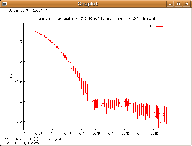
 Run title:  Lysozyme, high angles (>.22) 46 mg/ml, small angles (<.22) 15 mg/
 Number of points in the run is  196
 Input data, second file               [ none        ] :
 No of end points to omit              [    0        ] :
 Total number of input data points read is  196
 Angular range as read: from  0.04138   to  0.49603
 Angular scale (1/2/3/4)               [    1        ] :
 Plot input data                 (Y/N) [   Yes       ] :

Press CR to continue
 File containing expert parameters     [ none        ] :
 Kernel already calculated       (Y/N) [   No        ] :
 Type of system        (0/1/2/3/4/5/6) [    0        ] :
 Zero condition at r=rmin        (Y/N) [   Yes       ] :
 Zero condition at r=rmax        (Y/N) [   Yes       ] :
   --  Arbitrary monodisperse system  --
  Rmin=0,  Rmax is maximum particle diameter
 Rmax for evaluating p(r)                              : 50
 Number of points in real space        [    101      ] :
 Kernel-storage file name              [ kern.bin    ] :
 Experimental setup            (0/1/2) [    0        ] :
 Evaluating design matrix. Please wait...

 Evaluating stabilizer matrix. Please wait ...
  The measure of inconsistency AN1 equals to    0.3345E+00
 Initial ALPHA                         [   0.0       ] :
Press CR to continue
     Alpha    Discrp  Oscill  Stabil  Sysdev  Positv  Valcen    Total
  0.1066E+01  0.3035  1.3523  0.0216  0.9436  1.0000  0.9391  0.88205

 Plot results                    (Y/N) [   Yes       ] :
Press CR to continue

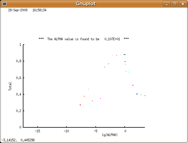
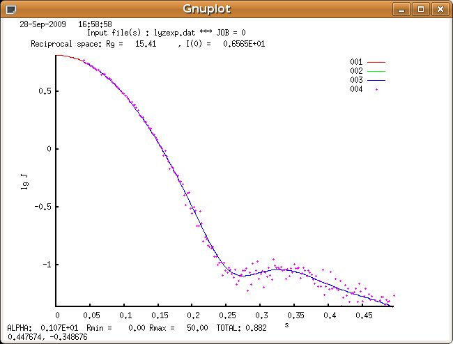
First plot shows how quality estimate varies with different ALPHA:

Next there is a reciprocal space fit of scattering computed for final P(r) function to data:

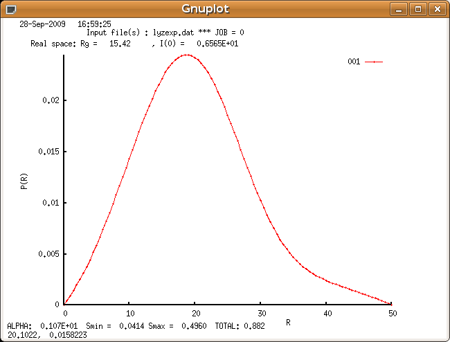
Finally it plots computed distribution function P(r):

Press CR to continue
 Parameter    DISCRP    OSCILL    STABIL    SYSDEV    POSITV    VALCEN
 Weight        1.000     3.000     3.000     3.000     1.000     1.000
 Sigma         0.300     0.600     0.120     0.120     0.120     0.120
 Ideal         0.700     1.100     0.000     1.000     1.000     0.950
 Current       0.304     1.352     0.022     0.944     1.000     0.939
                - - - - - - - - - - - - - - - - - - - - - - - - -
 Estimate      0.174     0.838     0.968     1.000     1.000     0.992

  Angular   range    :     from    0.0414   to    0.4960
  Real space range   :     from      0.00   to     50.00

  Highest ALPHA (theor) :   0.315E+01                 JOB = 0
  Current ALPHA         :   0.107E+01   Rg :  0.154E+02   I(0) :   0.657E+01

           Total  estimate : 0.882  which is    A GOOD      solution

                 ===   Select one of the following options  ===
                     - - - - - - - - - - - - - - - - - - - -
                 CR     ---  to accept the solution and   EXIT
            -(NewAlpha) ---  to manually change           ALPHA
           1,2,3,4,5,6  ---  to change weight/sigma of PARAMETERS
                  7     ---  to maximize a new  total   ESTIMATE
                  8     ---  to replot the              SOLUTION
 Your choice :
 Evaluating the final solution. Please wait ...
 Evaluate errors                 (Y/N) [   Yes       ] :
 Monte-Carlo simulations. Please wait...

 Plot p(r) with errors           (Y/N) [   Yes       ] :

Press CR to continue
 Next data set           (Yes/No/Same) [   No        ] :

References

1. Feigin L.A. & Svergun D.I. (1987). Structure Analysis by Small-Angle X-Ray and Neutron Scattering. NY: Plenum Press.
2. Glatter O. (1977). J.Appl.Cryst., 10, 415-421
3. Moore P.B. (1980). J.Appl.Cryst., 13, 168-175
4. Provencher S.W. (1982). Computer Phys.Commun., 27, 213-227, 229-242
5. Svergun D.I., Semenyuk A.V. (1987). Doklady AN SSSR, 297, 1373-1377 (in Russian)
6. Svergun D.I., Semenyuk A.V., Feigin L.A. (1988). Acta Cryst., A44, 244-250
7. Svergun D.I. (1991). J.Appl.Cryst., 24, 485-492
8. Tikhonov A.N., Arsenin V.Ya. (1977). Solution of Ill-Posed Problems. NY: Wiley
9. Tikhonov A.N., Goncharsky A.V., Stepanov V.V., Yagola A.G. (1983). Regularizing Algorithms and a priory Information. Moscow: Nauka, (in Russian)
10. Svergun D.I. (1992). J. Appl. Cryst., 25, 495-503.