POLYSAS manual

Written by P.V. Konarev, V.V. Volkov, and D.I. Svergun.
Post all your questions about POLYSAS to the ATSAS Forum.

© ATSAS Team, 2012-2016

Table of Contents

• Manual
  • Introduction
  • POLYSAS User Interface
    • Menus and Dialogs
  • Using POLYSAS
    • Loading data
    • Plotting data
    • Determine overall structural parameters and invariants
    • Calculation of size distributions
    • Fitting the data with pdb models
    • Analysis of mixtures using pdb models
    • Analysis of mixtures using geometrical models
    • SVD anlysis: number of components

Manual

Introduction

Program POLYSAS is an interactive graphical system for small-angle scattering analysis of polydisperse systems and multiple data sets. POLYSAS has a menu-driven graphical user interface calling computational modules from ATSAS package to perform data treatment and analysis. The graphical menu interface allows one to process multiple (time, concentration or temperature-dependent) data sets and interactively change the parameters for the data modeling using sliders. The graphical representation of the data is done via the Winteracter-based program SASPLOT. The package is especially suited for the analysis of polydisperse systems and mixtures, and permits to obtain size distributions and evaluate the volume fractions of the components using linear and non-linear fitting algorithms as well as model-independent singular value decomposition.

POLYSAS is compiled using Intel Visual Fortran v.11.0 and runs under MS Windows XP/7/8 or under Windows emulators (like WINE) installed on Linux/MAC.

If you use the results from POLYSAS in your own publication, please cite:

P.V.Konarev, V.V.Volkov, and D. I. Svergun (2016). Interactive graphical system for small-angle scattering analysis of polydisperse systems. Journal of Physics: Conference Series. 747, 012036

POLYSAS User Interface

Menus and Dialogs

Menu options	Description
Load experimental data sets	This menu option allows one to select and load multiple data sets (from time-, concentration- or temperature-dependent serias of measurements), plot data within the pre-selected angular range, and estimate overall structural parameters (radius of gyration Rg, maximum size of the particle Dmax, excluded (Porod) volume of the particle) for the entire data set.
Size distribution	Menu permits to calculate distance and size distribution functions for monodisperse and polydisperse systems of particles of different types (spheres, hollow spheres, rod and flat particles).
Choose model	Menu contains options for multi-type analysis of polydisperse systems, using the fits from pdb models, analysis of oligomeric mixtures and interactive polydisperse systems using geometrical bodies as well as model-independent estimation of number of components using singular value decomposition.
Help	Menu contains short information the program and the link to ATSAS sasdoc help program with the manual descriptions of the ATSAS programs.

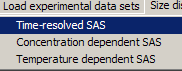
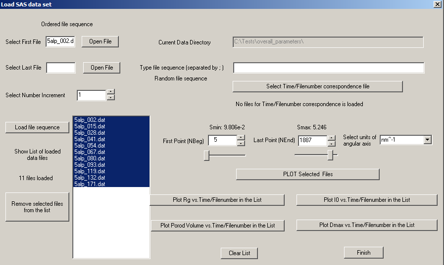
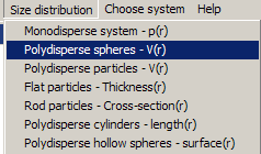
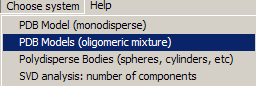
Using POLYSAS

Loading data

One can load the data using "SELECT" or "LOAD FILE SEQUENCE" of the corresponding dialogs. The first case corresponds to the single curve loading, the second case - to the multiple curve loading.

For convenient and fast multiple file selection using 'LOAD FILE SEQUENCE' button one has to pre-specify the values for "First file" ( for example "xxxx_001" ) and for "Last file" ( for example "xxx_007") and the Number Increment (the increment in the run numbers to be selected) in the dialog box. If the edit box for the "Last File" is empty then the program will automativcally look for all files beginning from "xxx_NNN"-"First File" up to "xxx_999" and will choose only existing files. It works also for the files with four and five digits at the end of file names (e.g. xxx_00001 or xxx_00001.dat). It is also possible to use wild file name masks for the 'First File' box, e.g. one can specify there 'xxx*.dat' value and then all files starting with 'xxx' and having extension 'dat' will be automatically loaded. There is also an option to select the sequence of files with completely random namings using 'Type file sequence (Random file sequence)' dialog box. In the latter case one has to write the file names separated by ';' symbols. The specified files should be present in the 'Current Data Directory' which is shown in inactive layout on the top of the dialog.

After the files were loaded one can use the buttons 'Remove selected file from the list' and 'Clear List' in order to manipulate with the loaded data sets. For the first case one needs to select the file to be removed from the list and then press the 'Remove' button, in the second case ('Clear List' button) all loaded files will be removed.

Plotting data

After loading the data one can use the buttons 'PLOT Selected Files' or 'Plot Data'/'Plot experimental data'. The program SASPLOT will be called and it will make a graph of the corresponding data sets in the data range specified within 'First Point' and 'Last Point' dialog boxes. One can use sliders or spin buttons in order to change interactively the angular range of the selected data. The units of the angular axis can be defined as inverse Angstroem or inverse nanometers, the corresponding values will be shown on the s-axes of the graphs.

Determine overall structural parameters and invariants

For multiple data sets one can estimate the following overall parameters:

1) Rg dependence - with 'Plot Rg vs. Time/FileNumber in the List' button

2) I0 dependence - with 'Plot I0 vs. Time/FileNumber in the List' button

3) Dmax dependence - with 'Plot Dmax vs. Time/FileNumber in the List' button

4) Porod Volume dependence - with 'Plot Porod Volume vs. Time/FileNumber in the List' button

After clicking on one of these buttons, the program will subsequently estimate the corresponding parameters (using DATRG, DATGNOM and DATPOROD from ATSAS package) accoring to the order of the loaded data file list, the progress of the calculation will be shown in the information window, the SASPLOT window plot will be automatically updated when the next data file in the list is being processed. It is recommended not to interrupt the calculations/ re-plotting of the data during the file list processing.

There is also an option to pre-select the corresponding dependence of the time (concentration or temperature) vs. filenumber in the selected file list using 'Select Time/Filenumber corresponding file' where one needs to specify in ASCII format using two-column format the correspondence between filenumbers in the list and the dependent parameter value (ms or s for time, mg/ml for concentration or degrees for temperature). Then the units of the s-axis in the graph plots will be automatically tranformed into the data-dependent parameters.

Calculation of size distributions

The submenus of the main 'Size distribution' menu correspond to different system types of the particles (that exactly correspond to JOB type parameter in GNOM program starting from 0 to 6). One can select the corresponding submenu and then estimate the size distribution for the selected system type. For this one needs to select the experimental data file using the 'Select' button and then press 'Evaluate Distribution' button. The plot of the experimental data and its fit from GNOM program will be displayed in the top-right corner of the screen whereas the corresponding size distribution function will be shown in the bottom-right corner of the screen.

To see the log information from GNOM run one needs to press 'Show GNOM summary' button, here you can find the estimations of the TOTAL parameter in GNOM and the corresponding contributions from different criteria used in GNOM.

The user can interactively change the parameters using the sliders and the spin buttons in the dialog window for the Indirect Fourier Transformation (IFT) analysis in GNOM (such as Rmin/Rmax-Dmax, the smoothness Alpha parameter, Number of points for P(r)/V(r) functions and experimental setups with the corresponding parameters responsible for experimental data smoothing). The updated plots will be automatically redrawn. For more details on IFT analysis see GNOM manual.

It is recommended always to work with one type of dialog at one time and do not open simultanuously different dialogs, it can lead to mixing up of the results/plots. Before closing the dialog with 'Finish' button it is safer to press 'Clear' button in order to empty the selected file list so that it will not appear in another type of dialogs when one starts a different model approach.

Fitting the data with pdb models

This dialog is designed for fast calculation of the theoretical data curves from the selected pdb models (from the loaded file list) and for the fitting them to the experimental data curve. CRYSOL from ATSAS package will be called and the results will be displayed via SASPLOT. With the button 'Run CRYSOL against experimental data' you will get the fits to ALL loaded PDB models, each fit will be plotted in a separate window.

The user can also interactively change using the sliders and the spin buttons in the dialog box the parameters for the CRYSOL calculations, such as maximum S-value (Smax), the maximum number of spherical harmonics (Lm), the number of points in the theoretical curves and the constant subtraction during the fitting of experimental data.The button 'Plot latest CRYSOL fit from selected PDB' permits to display the latest fit from CRYSOL for the selected PDB (all subsequent fits from CRYSOL has an increasing numbering, such as fileName00.fit, fileName01.fit etc.)

One can use 'Show CRYSOL Log file' to display the information from CRYSOL calculations'. It is recommended to press 'Clear' and then 'Finish' buttons when finishing the modelling.

Analysis of mixtures using pdb models

The dialog permits one to fit experimental data seria with the linear combinations of the scattering curves calculated from the selected PDB models. The volume fractions of the components in the oligomeric mixtures are calculated using the program OLIGOMER (from ATSAS package) and the results are displayed via SASPLOT.

The graph with the theoretical curves calculated from PDB models will be displayed in the top-right corner of the screen, the graph with the fits to the experimental data seria is shown in the bottom-right corner of the screen, the graph with the volume fractions of the components is displayed in the bottom-left corner.

There are similar to the previous section (fits with PDB models) options, namely one can interactively change the parameters for the calculations of the theoretical curves from the selected PDB files and show the log file from OLIGOMER calculations with the values of the volume fractions and the corresponding fit quality values.

Analysis of mixtures using geometrical models

This dialog can be used for the non-linear analysis of the multi-component systems using the simple geometrical bodies (of three types: spheres, cylinders and dumb-bells and for maximum five components) and taking into account the polydispersity effects and interparticle interactions (the latter can be applied for the spherical particles only using the approximation of sticky hard sphere potential).

The parameters of the models can be interactively changed using the sliders and spin buttons and the fit from the current model to the experimental data curve can be calculated using the button 'Evaluate current model'.

One can define the upper and lower limits as well as fixation of the parameters for each 'phase'-component inside 'Define Boundaries for #N' buttons. Then by pressing the button 'Optimize current model' one can start the minimization process (calculated by the program MIXTURE from ATSAS package), when the minimization is finished, the results of the fits and partial intensities from the components will be shown via SASPLOT.

The graph with the fit to the experimental data will be displayed in the top-right corner of the screen, the graph with the partial intensities from the components is shown in the bottom-right corner of the screen, the graph with the structure factor for the spherical particles is displayed in the bottom-left corner.

The log file from MIXTURE with the optimized parameters can be shown via the 'Show Log file' button.

SVD analysis: number of components

With this dialog one can estimate the number of components in the system measured at different conditions (at different pH, temperature, buffer type, sample and salt concentration, ligand addition etc.). The model independent singular-value decomposition is used in the calculations, namely via the program SVDPLOT from ATSAS package.

There are options to estimate the eigenvectors and the egenvalues of SVD decompositions for the entire data set (with the buttons 'Plot Eigenvalues/Eigenvectors for full subset') or only for the selected subset of the data curves (with the buttons 'Plot Eigenvalues/eigenvectors for selected subset'). The estimated number of components from SVDPLOT will be shown in the information window below the dialog box.